Breadcrumbs
How to use Quick Analysis in Excel 2013
Description: To quickly change formatting, make charts, get totals, create tables, or insert sparklines you can access the quick analysis menu to perform these actions efficiently.
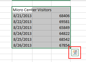
- When you have data in a spreadsheet and you want to quickly make a change to it, whether it be changing the formatting, making charts, getting totals, creating tables or inserting sparklines, all you have to do is highlight the data set, then in the bottom right hand corner you will see a box appear - click on that box.
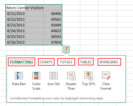
- This will open the Quick Analysis menu where you can select formatting, charts, totals, tables, and sparklines.
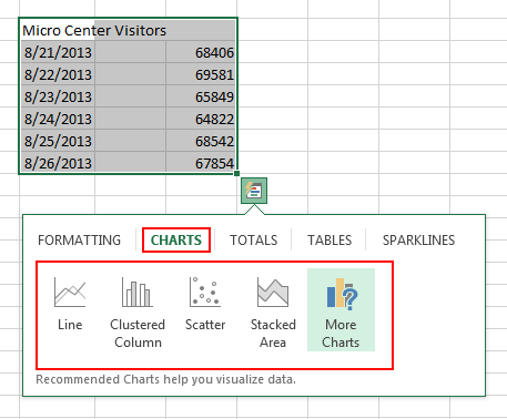
- For this example let's select charts. This gives us some options to choose from, the selection will be the most popular chart types, if you do not see your chart type click on more charts.
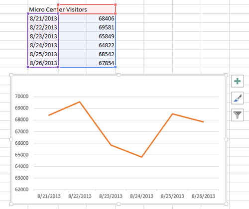
- Let's select the line chart. You will notice when you hover your mouse over line chart you will get a preview of what it will look like.
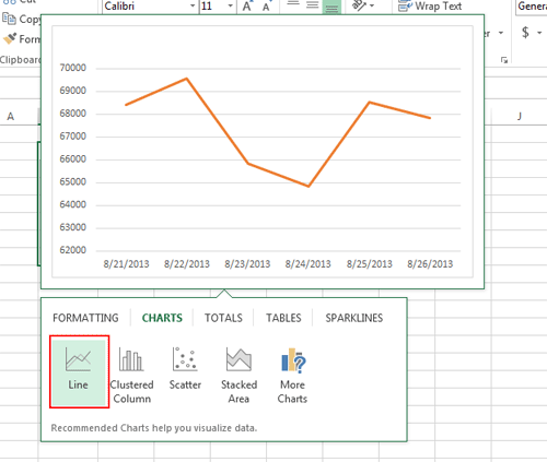
- After you have picked a chart type, click on it to insert the chart into the spreadsheet.
Technical Support Community
Free technical support is available for your desktops, laptops, printers, software usage and more, via our new community forum, where our tech support staff, or the Micro Center Community will be happy to answer your questions online.
Forums
Ask questions and get answers from our technical support team or our community.
PC Builds
Help in Choosing Parts
Troubleshooting
